
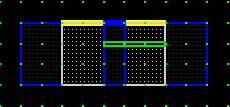
Top View
Side View
The antenna consists of a simple rectangular patch, and is modeled as an infinitely-thin perfect conductor. The antenna is excited from beneath via a round coaxial feed.
To obtain the performance characteristics of the antenna, two models were built and simulated. The first model is a continuous coaxial conductor alone, to serve as a reference. The second is the full model, containing the patch on top of a dielectric substrate and the coaxial feed beneath. The full model result is normalized by the reference model result to obtain the S-parameter response of the structure.
Thanks to Keith Kelly and Ian Rumsey of
Ball Aerospace & Technologies
for providing this example.
Both the center conductor and the teflon insulator are modeled with
circular cross-section.
In the simulation, the center conductor occupies a single
(square) grid cell, due to the coarse grid resolution.
The teflon insulator is staircased in a similar fashion.
If the grid cell size was even larger, the simulated center conductor
would degenerate into an infinitely-thin wire.
This representation may still result in an accurate simulation.
However, if the teflon insulator is meshed too coarsely, it may
degenerate completely, resulting in the outer conductor shorting
with the inner conductor in the simulated model.
As shown in the model top view, there are two cells of teflon around
the outside of the center conductor.
This leaves sufficient separation to prevent the teflon region from
degenerating, and even approximates the circular cross-section.
Two probes are also added to the model to record the response.
A current probe is positioned on top of the source region, and
a voltage probe is placed between the two conductors.
The PML absorbing boundary condition has been used to absorb the
signal as it moves along the center conductor and to the edge
of the grid, effectively extending the model indefinitely without
discontinuity.
Feed Reference Model Geometry
The feed reference model is very simple, with a wire extending through
the center of a teflon-filled hole in the outer conductor.
The wire is excited by an LC current source, which is simulated as
a current loop around the conductor.
The current source is defined to wrap closely around the wire, which
results in the loop excitation one-half of a cell outside the wire,
within the teflon insulator.
|
Top View |
Side View |
In the images, metal is shown in blue, teflon in yellow and gray, and the
probe regions as green.
Patch Model Geometry
The patch model adds a dielectric substrate on top of the coaxial conductor,
which has been extended to provide a ground plane.
The center conductor of the coax extends up through the dielectric layer
and makes contact with the patch.
A region of air has been added above the patch to allow it to radiate.
 |
A close-up side view of the patch model.
The current source along the coax has been red/white highlighted. |
Again the PML absorbing boundary condition has been used, to prevent reflection
of the energy radiated by the patch from re-entering the probe region.
Model Excitation
A smart choice for the current source waveform can reduce the
amount of computation required to run the simulation by
limiting the number of time steps needed.
In this model, a modulated gaussian pulse with a center frequency
of 9 GHz is used.
A high (1/e) frequency of 15 GHz is set to provide a large bandwidth.
This is useful so that a wideband result can be obtained.
This source requires 477 time steps.
After the excitation is complete, more time steps are needed to
allow the signal to propagate through and radiate from the antenna.
 |
A frequency domain view of the modulated gaussian source waveform.
The same excitation is used for both the reference model and the patch model. |

|
The current flowing along the center conductor calculated in the patch model simulation. |
 |
The current flowing along the center conductor calculated in the reference model simulation. |
 To calculate the impedance of the coax feed, the values recorded by the
voltage and current probes are used.
An LC pulse is defined in the Define Pulses dialog, coupling
the voltage and current probes together.
Then the Step Pulses dialog is used to display the results
from the pulse calculation.
For this structure, an impedance of 44 ohms is obtained.
To calculate the impedance of the coax feed, the values recorded by the
voltage and current probes are used.
An LC pulse is defined in the Define Pulses dialog, coupling
the voltage and current probes together.
Then the Step Pulses dialog is used to display the results
from the pulse calculation.
For this structure, an impedance of 44 ohms is obtained.

|
This plot shows the reference probe (red), the patch probe (blue), and the reflected waveform (green). |

|
The reference probe is red, and the reflected waveform (diff_f) is blue. |
Sometimes the Define Calculations dialog can be used to avoid having to create dummy probes. An LC calculation is an algebraic combination of one or more probes within a simulation. Since the reflected waveform was created from a calculation involving probe data from two different simulations, Define Calculations can't be used.

Another way to do this same calculation is to use the
Plot S-Parameters dialog, only selecting S11.
Again, since we are combining data from two different simulations,
this feature can't be used as designed.
It's possible to use the dummy probe and pulse definition created
earlier along with the reference pulse to obtain S11.
Reducing the cell size would improve the geometric fidelity, which is
especially lacking in the round coax.
The memory required for the simulation rises dramatically as the
cell size decreases, so this approach has practical limits.
Also, since the time step size is proportional to the cell size, more
time steps are required for a model resolved with a finer mesh to
reach the same point in simulated time.
This effect can be somewhat reduced by tuning the source excitation.
Running the patch model for a longer time would include still more
of the patch response in the final solution.
Although the ringing had been reduced substantially by 3000 time steps,
the variation was still visible in the plots; this is a visual clue that
some error has been tolerated in the interest of a shorter run time.
By including more simulated time, the ripple in the reflected waveform
frequency domain plot (and the S11 plot) can be reduced.
Can These Results Be Improved?
Both increasing the mesh density (i.e., reducing the cell size) and
running the simulation for a longer time would improve on the results.

|
S11 calculated after 10000 time steps.
A much sharper and deeper resonance is apparent. |