HyperFun for Windows: Graphics and Animation
Static images
The images below (except the isosurface) are generated using the following model:
fsin(x[2], a[1]){
d=x[1]^2+x[2]^2;
fsin = sin(d)*exp(-sqrt(d));
}
The table below shows the available image types and corresponding assignement
of coordinates X Assign and function F Assign.
Click on an image below to get its larger size version.
|
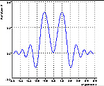
Plot y=f(x,c)
x[1] -> X axis
x[2] -> 0
f -> Y axis
|
|
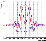
Group plot y=f(x,ci)
x[1] -> X axis
x[2] -> Group value
f -> Y axis
|
|
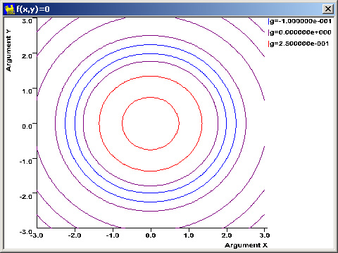
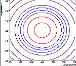
Contour line f(x,y)=c
x[1] -> X axis
x[2] -> Y axis
f -> 0
|
|
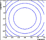
Contour map f(x,y)=ci
x[1] -> X axis
x[2] -> Y axis
f -> Group value
|
|
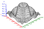
Surface z=f(x,y)
x[1] -> X axis
x[2] -> Y axis
f -> Z axis
|
|
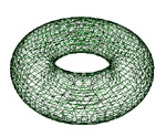
Isosurface f(x,y,z)=c
x[1] -> X axis
x[2] -> Y axis
x[3] -> Z axis
f -> 0
(see model below)
|
The isosurface above is generated using the model:
torus(x[3], a[1]){
array center[3];
center = [0, 0, 0];
torus = hfTorusY(x,center,7,3);
}
Animation
The above image types can be time-dependent with using mapping of an additional coordinate to a Time variable.
For example, for the model:
fsin(x[3], a[1]){
d=x[1]^2+x[2]^2;
fsin = sin(d+x[3])*exp(-sqrt(d));
}
Define a time-dependent plot y=f(x,t):
x[1] -> X axis
x[2] -> 0
x[3] -> T1 time variable
f -> Y axis
Define the Time Curve for x[3]
Generate animation (AVI, 410K).
Back to HyperFun Tools page